The Steady State Genetic Algorithm and The Evolution Strategy Comparison
Hello, Friends!!
I read something about Generation Gap, Overlapping Populations and Steady State Genetic Algorithm (SSGA), so, I decided to implement those stuffs and try some comparison between them and the Evolution Strategy.
Here we have the configurations of the SSGA and the Evolution Strategy (ES):
Steady State Genetic Algorithm (SSGA):
String Length: 25 bits
Parents Population: 100
Generation Gap: 70
Crossover Probability: 0.7
Mutation Probability: 0.03
Elitism: Highly Elitist
Number of Generations: 3000
NOTE: The Generation Gap above means that only 70 parents can reproduce, that is, they generate 70 offspring and, after the reproduction, both parents population and offspring population compete for survival, i.e., we have a post-selection in wich from the temporary population parents+offspring we select the best 100 individuals to compose the next generation.
Evolution Strategy (ES):
Type of ES: (mu + lambda)-ES
Number of Parents(mu): 15
Number of Offspring(lamdba): 35
Mutation: O.k
Crossover: O.k
Number of Generations: 30; 45; 1000
1-First Function: Schwefel Function
F1 = sum(-x(i)·sin(sqrt(abs(x(i))))), i=1:2
x(1) = [-500:500]
x(2) = [-500:500]
Global Minimum: 837.9658; x(i)=420.9687, i=1:2
Here we can see an image of Schwefel's Function:

This function is deceptive and the search for the global minimum can drive the search to a wrong direction.
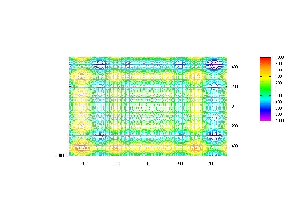
Below there is a contour map of the Schwefel Function.

SSGA
Best Initial Values
x1 = 404.66612293321259
x2 = -274.55141468499346
F(x1,x2) = -594.4647574012356
Best Final Values (after 3000 Generations)
x1 = 420.96873882319744
x2 = 420.96903684643019
F(x1,x2) = -837.96577453421264
Simulation Time = 83.61 s
Evolution Strategy
Best Initial Values
x1 = -339.01782978280346
x2 = 405.52768712189408
F(x1,x2) = -532.95484456153542
Best Final Values (after 30 Generations)
x1 = 420.96873130520726
x2 = 420.96870632616128
F(x1,x2) = -837.96577454463647
Simulation Time = 0.04 s
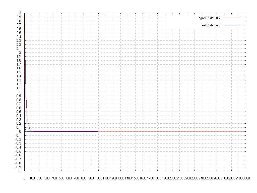
Here we have a performance comparison of the best fitness versus generation (the Blue Line is the Evolution Strategy and the Red Line is the Steagy State Genetic Algorithm):

As we can see, both SSGA and the ES could achieve the global minimum and, althoug the SSGA seems, at a first glance, have spent much more time than the ES, in the graph above we note that the SSGA got a solution very close to that achivied by the ES, and for this the SSGA did not spent so much generations.
2-Second Function: Schaffer Function
Number of Variables: 2
Number of optima: 1
Variables' Range: x1 = x2 = [-100:100]
Optima Variables: x1 = x2 = 0
Optimum Function Value: f(x1,x2) = 0
SSGA
Best Initial Values
x1 = -3.1670779933654662
x2 = -6.9732697896143732
F(x1,x2) = 2.9646431665317086
Best Final Values (after 3000 Generations)
x1 = -2.9802323275873732e-006
x2 = 2.9802323275873732e-006
F(x1,x2) = 0.0036238913066679486
Simulation Time = 61.629 s
Evolution Strategy
Best Initial Values
x1 = 8.4105629978750667
x2 = 7.3227216058050848
F(x1,x2) = 4.6930491714630076
Best Final Values (after 1000 Generations)
x1 = 1.3362218153590791e-162
x2 = -2.8625317383361051e-163
F(x1,x2) = 0
Simulation Time = 1.232 s
Here a comparison.

3 - Third Function: Easom Function
Number of Variables: 2
Number of optima: 1
Variables' Range: x1 = x2 = [-100:100]
Optima Variables: x1 = x2 = pi
Optimum Function Value: f(x1,x2) = -1
SSGA
Best Initial Values
x1 = -11.977538823412026
x2 = 1.2930781034552485
F(x1,x2) =-3.975239915042439e-102
Best Final Values (after 3000 Generations)
x1 = 3.141591046499939
x2 = 3.1415970069645942
F(x1,x2) = -0.99999999996769862
Simulation Time = 58.173 s
Evolution Strategy
Best Initial Values
x1 = 21.300842203805615
x2 = 14.823566430631823
F(x1,x2) = -1.6190289343389992e-203
Best Final Values (after 45 Generations)
x1 = 3.1415926565055088
x2 = 3.1415926519644986
F(x1,x2) = -1
Simulation Time = 0.061 s
The Graph:

One more time the ES got a very good solution and the SSGA did not find the result, althoug the SSGA is very close to it. The ES was faster and the most important: the ES got the solution using only 45 generations.
4 - Fourth Function: Michalewicz Function
Number of Variables: 2
Number of optima: 1
Variables' Range: x1 = x2 = [0:pi]
Optima Variables: x1 = x2 = pi/2
Optimum Function Value: f(x1,x2) = -2
SSGA
Best Initial Values
x1 = 1.5210479820083809
x2 = 1.4612604610821343
F(x1,x2) = -1.5408508750355414
Best Final Values (after 3000 Generations)
x1 = 1.5707963736082748
x2 = 1.5707963736082748
F(x1,x2) = -1.9999999999999993
Simulation Time = 55.8 s
Evolution Strategy
Best Initial Values
x1 = 1.7029091414282871
x2 = 1.6858213688002974
F(x1,x2) = -1.0194035697340043
Best Final Values (after 35 Generations)
x1 = 1.5707963223628052
x2 = 1.5707963300574828
F(x1,x2) = -2
Simulation Time = 0.03 s
The Graph:

5 - Fifth Function: Ackley's Function
F5 = -a·exp(-b·sqrt(1/n·sum(x(i)^2)))-exp(1/n·sum(cos(c·x(i))))+a+exp(1)
a=20; b=0.2; c=2·pi; i=1:2
x1 = [-32.768:32.768]
x2 = [-32.768:32.768]
Global Minimum: f = 0; x1 = x2 = 0;
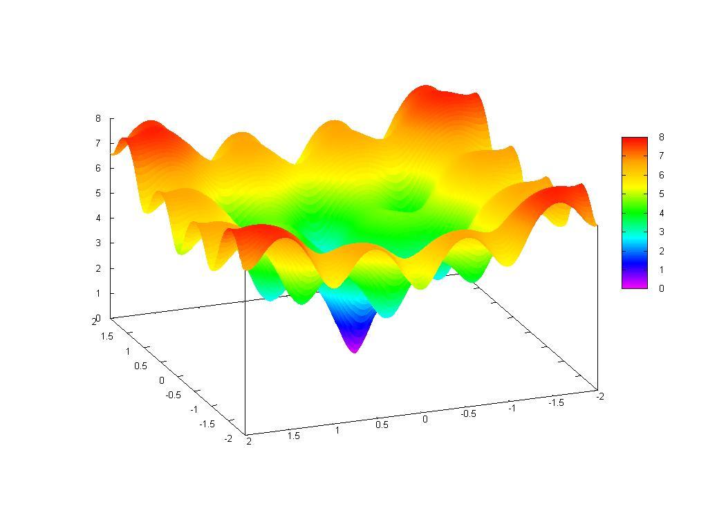
Below we can see the graph of Ackley's Function:
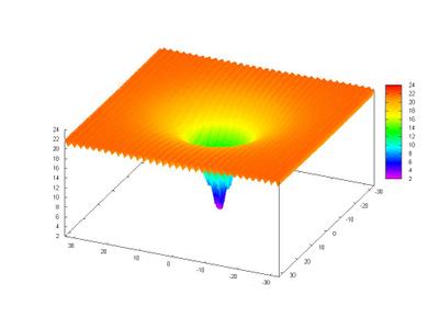
This function is very multimodal, there are a lot of local optima, and this can trap the search in those places.
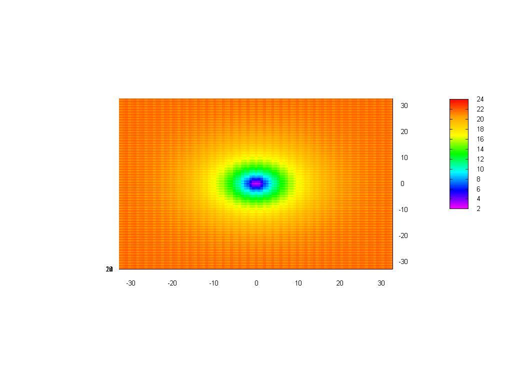
A closer view:

A plot map:

SSGA
Best Initial Values
x1 = -1.0377881168659961
x2 = -2.285001044660838
F(x1,x2) = 7.2358656827208128
Best Final Values (after 3000 Generations)
x1 = -9.7656252910291452e-007
x2 = 9.7656252910291452e-007
F(x1,x2) = 3.9063009055542979e-006
Simulation Time = 70.251 s
Evolution Strategy
Best Initial Values
x1 = 2.7559732831437018
x2 = 2.3995094157902104
F(x1,x2) = 10.108951936627786
Best Final Values (after 1000 Generations)
x1 = 1.0133584085863174e-016
x2 = 2.3441664160783457e-017
F(x1,x2) = 1.4463256980956629e-016
Simulation Time = 1.272 s
A comparison:

Well, I think that both were not so good in the search, the global minimum was not achivied with a good precision.
We saw, again, that the ES had a better performance than the SSGA, I do not know if this is due the kind of problem that each one was designed to deal or, simply, because the ES is better in those kind of problems.
Até Mais!!!
Marcelo
I read something about Generation Gap, Overlapping Populations and Steady State Genetic Algorithm (SSGA), so, I decided to implement those stuffs and try some comparison between them and the Evolution Strategy.
Here we have the configurations of the SSGA and the Evolution Strategy (ES):
Steady State Genetic Algorithm (SSGA):
String Length: 25 bits
Parents Population: 100
Generation Gap: 70
Crossover Probability: 0.7
Mutation Probability: 0.03
Elitism: Highly Elitist
Number of Generations: 3000
NOTE: The Generation Gap above means that only 70 parents can reproduce, that is, they generate 70 offspring and, after the reproduction, both parents population and offspring population compete for survival, i.e., we have a post-selection in wich from the temporary population parents+offspring we select the best 100 individuals to compose the next generation.
Evolution Strategy (ES):
Type of ES: (mu + lambda)-ES
Number of Parents(mu): 15
Number of Offspring(lamdba): 35
Mutation: O.k
Crossover: O.k
Number of Generations: 30; 45; 1000
1-First Function: Schwefel Function
F1 = sum(-x(i)·sin(sqrt(abs(x(i))))), i=1:2
x(1) = [-500:500]
x(2) = [-500:500]
Global Minimum: 837.9658; x(i)=420.9687, i=1:2
Here we can see an image of Schwefel's Function:

This function is deceptive and the search for the global minimum can drive the search to a wrong direction.
Below there is a contour map of the Schwefel Function.
SSGA
Best Initial Values
x1 = 404.66612293321259
x2 = -274.55141468499346
F(x1,x2) = -594.4647574012356
Best Final Values (after 3000 Generations)
x1 = 420.96873882319744
x2 = 420.96903684643019
F(x1,x2) = -837.96577453421264
Simulation Time = 83.61 s
Evolution Strategy
Best Initial Values
x1 = -339.01782978280346
x2 = 405.52768712189408
F(x1,x2) = -532.95484456153542
Best Final Values (after 30 Generations)
x1 = 420.96873130520726
x2 = 420.96870632616128
F(x1,x2) = -837.96577454463647
Simulation Time = 0.04 s
Here we have a performance comparison of the best fitness versus generation (the Blue Line is the Evolution Strategy and the Red Line is the Steagy State Genetic Algorithm):

As we can see, both SSGA and the ES could achieve the global minimum and, althoug the SSGA seems, at a first glance, have spent much more time than the ES, in the graph above we note that the SSGA got a solution very close to that achivied by the ES, and for this the SSGA did not spent so much generations.
2-Second Function: Schaffer Function
Number of Variables: 2
Number of optima: 1
Variables' Range: x1 = x2 = [-100:100]
Optima Variables: x1 = x2 = 0
Optimum Function Value: f(x1,x2) = 0
SSGA
Best Initial Values
x1 = -3.1670779933654662
x2 = -6.9732697896143732
F(x1,x2) = 2.9646431665317086
Best Final Values (after 3000 Generations)
x1 = -2.9802323275873732e-006
x2 = 2.9802323275873732e-006
F(x1,x2) = 0.0036238913066679486
Simulation Time = 61.629 s
Evolution Strategy
Best Initial Values
x1 = 8.4105629978750667
x2 = 7.3227216058050848
F(x1,x2) = 4.6930491714630076
Best Final Values (after 1000 Generations)
x1 = 1.3362218153590791e-162
x2 = -2.8625317383361051e-163
F(x1,x2) = 0
Simulation Time = 1.232 s
Here a comparison.
3 - Third Function: Easom Function
Number of Variables: 2
Number of optima: 1
Variables' Range: x1 = x2 = [-100:100]
Optima Variables: x1 = x2 = pi
Optimum Function Value: f(x1,x2) = -1
SSGA
Best Initial Values
x1 = -11.977538823412026
x2 = 1.2930781034552485
F(x1,x2) =-3.975239915042439e-102
Best Final Values (after 3000 Generations)
x1 = 3.141591046499939
x2 = 3.1415970069645942
F(x1,x2) = -0.99999999996769862
Simulation Time = 58.173 s
Evolution Strategy
Best Initial Values
x1 = 21.300842203805615
x2 = 14.823566430631823
F(x1,x2) = -1.6190289343389992e-203
Best Final Values (after 45 Generations)
x1 = 3.1415926565055088
x2 = 3.1415926519644986
F(x1,x2) = -1
Simulation Time = 0.061 s
The Graph:
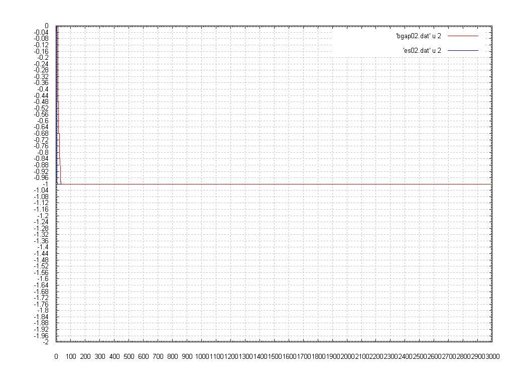
One more time the ES got a very good solution and the SSGA did not find the result, althoug the SSGA is very close to it. The ES was faster and the most important: the ES got the solution using only 45 generations.
4 - Fourth Function: Michalewicz Function
Number of Variables: 2
Number of optima: 1
Variables' Range: x1 = x2 = [0:pi]
Optima Variables: x1 = x2 = pi/2
Optimum Function Value: f(x1,x2) = -2
SSGA
Best Initial Values
x1 = 1.5210479820083809
x2 = 1.4612604610821343
F(x1,x2) = -1.5408508750355414
Best Final Values (after 3000 Generations)
x1 = 1.5707963736082748
x2 = 1.5707963736082748
F(x1,x2) = -1.9999999999999993
Simulation Time = 55.8 s
Evolution Strategy
Best Initial Values
x1 = 1.7029091414282871
x2 = 1.6858213688002974
F(x1,x2) = -1.0194035697340043
Best Final Values (after 35 Generations)
x1 = 1.5707963223628052
x2 = 1.5707963300574828
F(x1,x2) = -2
Simulation Time = 0.03 s
The Graph:

5 - Fifth Function: Ackley's Function
F5 = -a·exp(-b·sqrt(1/n·sum(x(i)^2)))-exp(1/n·sum(cos(c·x(i))))+a+exp(1)
a=20; b=0.2; c=2·pi; i=1:2
x1 = [-32.768:32.768]
x2 = [-32.768:32.768]
Global Minimum: f = 0; x1 = x2 = 0;
Below we can see the graph of Ackley's Function:

This function is very multimodal, there are a lot of local optima, and this can trap the search in those places.
A closer view:
A plot map:
SSGA
Best Initial Values
x1 = -1.0377881168659961
x2 = -2.285001044660838
F(x1,x2) = 7.2358656827208128
Best Final Values (after 3000 Generations)
x1 = -9.7656252910291452e-007
x2 = 9.7656252910291452e-007
F(x1,x2) = 3.9063009055542979e-006
Simulation Time = 70.251 s
Evolution Strategy
Best Initial Values
x1 = 2.7559732831437018
x2 = 2.3995094157902104
F(x1,x2) = 10.108951936627786
Best Final Values (after 1000 Generations)
x1 = 1.0133584085863174e-016
x2 = 2.3441664160783457e-017
F(x1,x2) = 1.4463256980956629e-016
Simulation Time = 1.272 s
A comparison:
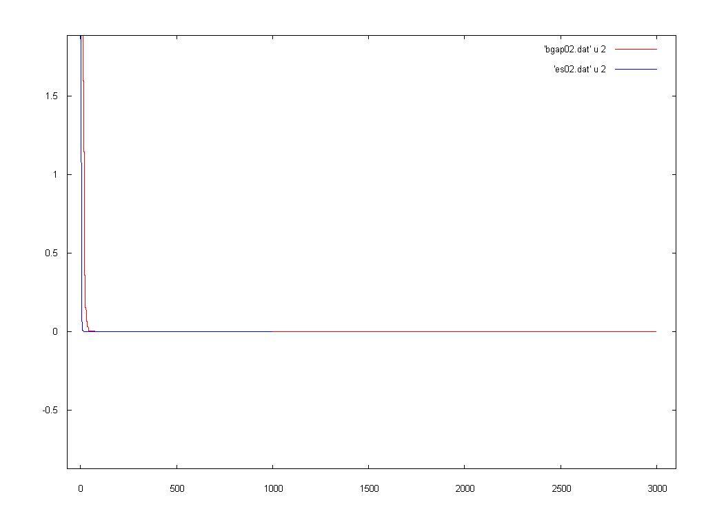
Well, I think that both were not so good in the search, the global minimum was not achivied with a good precision.
We saw, again, that the ES had a better performance than the SSGA, I do not know if this is due the kind of problem that each one was designed to deal or, simply, because the ES is better in those kind of problems.
Até Mais!!!
Marcelo
posted by Marcelo at 4:01 PM
9 comments
![]()


